PDEs and Finite Elements 
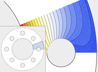
Mathematica Version 10 extends its numerical differential equation-solving capabilities to include the finite element method. Given a PDE, a domain, and boundary conditions, the finite element solution process - including grid and element generation - is fully automated. Stationary and transient solutions to a single PDE or a system of partial differential equations are supported for one, two, and three dimensions. Solve partial differential equations over arbitrarily shaped regions. » Solve stationary and transient PDEs in one, two, and three dimensions. Solve coupled systems of PDEs. Specify Dirichlet boundary conditions. » Specify generalized Neumann and Robin values. » Support for linear PDEs with coefficients that are variable in time and space. Freely formulate coupled PDEs for multiphysics analysis. Specify domains using the full geometric region framework. Fully automatic mesh generation from any region. Obtain solutions as approximate functions that can be further analyzed. Full suite of intermediate-level data structures and solution functions for detailed control and analysis of the solution. » Support for explicit mesh generation. Support for meshes with first- and second-order interpolation. Support for meshes with curved boundaries. Solve the Telegraph Equation in 1D » Solve a Wave Equation in 2D » Solve Axisymmetric PDEs » Solve PDEs over 3D Regions » Dirichlet Boundary Conditions » Neumann Values » Generalized Neumann Values » Solve PDEs with Material Regions » Transient Boundary Conditions » Transient Neumann Values » PDEs and Events » Solve a Complex-Valued Oscillator » Compute a Plane Strain Deformation » A Stokes Flow in a Channel » Structural Mechanics in 3D » Control the Solution Process »