


Control Systems
Since Mathematica 8, controls engineers can compute, analyze, and dynamically present control systems now. Besides comprehensive numeric methods, the symbolic features provide unexpected and uprecedented possibilities to simulate control tasks.
- State-space models
- Control systems with built-in symbolic computation capabilities
The components of these control system packages support computation in mechanics, electrical engineering, chemistry, aeronautical engineering, biology, and economics.
Analyze and design controls using classical techniques and state spaces, develop solutions for analog and digital systems, and simulate models in configurations with open and closed loops.
Some examples of control systems:
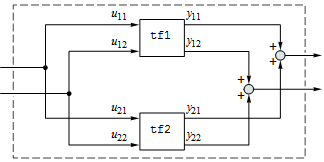
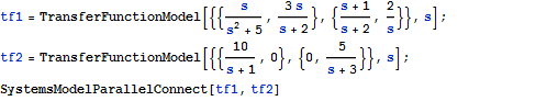
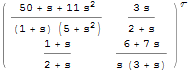
Zwei Parallelsysteme
Connect Two Systems in Parallel
Obtain the equivalent input-output model by connecting two systems in parallel.
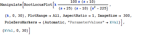
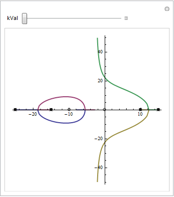
Interaktive Analyse
Interactively Analyze System Behavior
Determine critical points of system behavior, such as break-away, break-in, and imaginary-axis crossings, using an interactive root-locus plot.
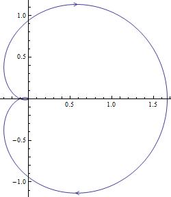
Systemstabilität
Determine System Stability Using Built-in Functions
Analyze a system's stability from its Nyquist plot.
![]()
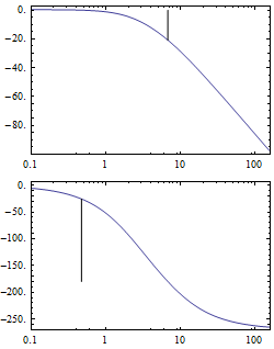
Visualisierungsmöglichkeiten
Visualize the Relative Stability of Systems
Gain and phase margins in a Bode plot.
![]()
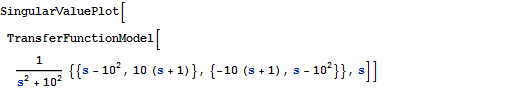
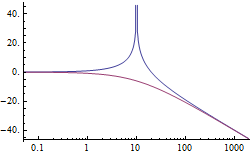
Frequenzgang
Study the Frequency Response of a Multivariable Systems
The singular value plot of a transfer-function model.
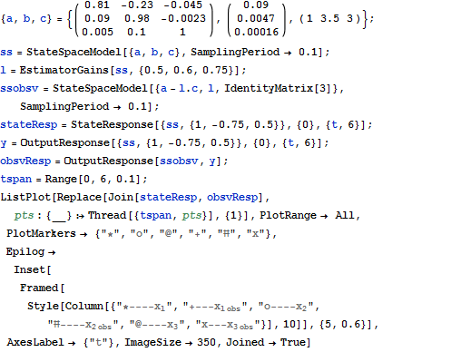
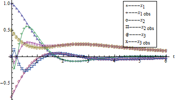
Beobachter und Regler
Build Regulators and Observers for Systems
The trajectories of the states and a Luenberger observer's state estimates.
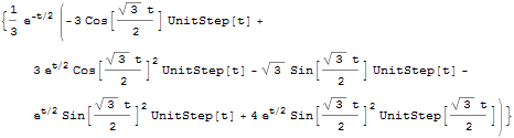
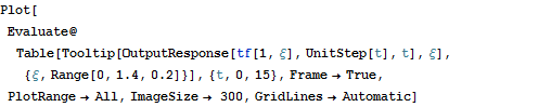
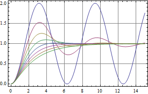
Simulation
Simulate the Response of State-Space or Transfer-Function Models
The step responses of a second-order system for different values of damping.
![]()
![]()
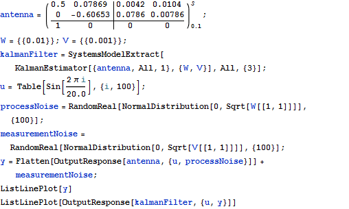
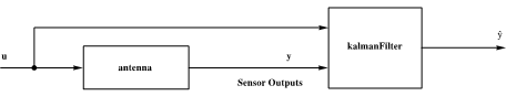
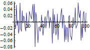
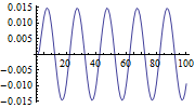
Kalman-Filter
Construct a Kalman Filter for a Stochastic System
Output of a system before and after optimal filtering.