What's New in GAUSS 18

Improved data handling

• NEW formula strings
• Read SAS and STATA datasets
• Improved Handling of Large Datasets

NEW formula strings simplify loading and transforming data

//Load data, transform and estimate in one step
call ols("credit.xlsx", "ln(balance) ~ ln(income) + factor(sex)");

//Load data, reclassifying string column 'state' into numerical categories
X = loadd("census.csv", "income + household_size + reclassify(state)");

GAUSS 18 expands the previously integrated formula string syntax to allow single line data loading, transformation, and analysis. The enhanced formula string syntax :

• Drastically decreases required lines of code.
• Works with CSV, Excel, GAUSS datasets, HDF5, SAS and STATA datasets.
• Supported automated transformations include:
  • apply transformations, such as `ln`, `exp` or any GAUSS procedure
  • create interaction terms
  • create dummy variables
  • reclassify string variables

Read SAS and STATA datasets

//Load SAS dataset, create interaction term and assign to GAUSS matrix 'X'
X = loadd("advertising.7bdat", "sales + radio * billboards + direct_mail");

//Load Stata dataset and compute descriptive statistics
call dstatmt("auto2.dta", "mpg + weight + gear_ratio");


Sharing data between GAUSS and other software just got easier. Not only does GAUSS 18 allow you to read SAS and STATA datasets, it also allows you to use SAS and STATA datasets directly as a dataset for functions such as OLS, GLM and the General Method of Moments.

• Complete compatibility with SAS and STATA datasets.
• Import SAS and STATA datasets as data matrices.
• Use SAS and STATA datasets as direct arguments in functions such as OLS, GLM and the GMM.

Improved Handling of Large Datasets

//Load large data in consecutive 1 GB blocks
setBlockSize("1G");

//Load large data in consecutive blocks no larger than 10% of system memory
setBlockSize("10%");

GAUSS 18 makes it easy to access and analyze large datasets with new, simple tools for controlling data processing. Users can now control data processing in terms of:

• Percentage of available memory.
• Simple memory specification.
• Number of rows.

General Method of Moments (GMM)

New GAUSS 18 GMM procedures estimate parameters from custom user specified moment equations or analytic instrumental variables estimates using one step, two-step, iterative, or continuously updating GMM.

Choose from two new GMM procedures!

• gmmFit provides full modeling flexibility including user-specified moment equations.
• gmmFitIV provides the analytic generalized method of moments estimates of instrumental variables models.

GAUSS GMM procedures provide new robust, efficient and customizable tools including:

• One-step, two-step, iterative, and continuously updating generalized method of moments estimation.
• Optional instrumental variables.
• Standard error and weight matrix options including standard, heteroskedastic robust, and HAC robust.
• Flexible initial weight matrix specification.

New Graphics Functionality

• New Color Palette Options and Defaults
• Control graph canvas size programmatically
• Other new features

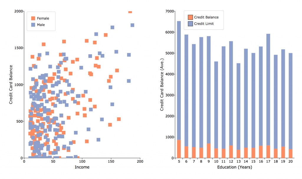
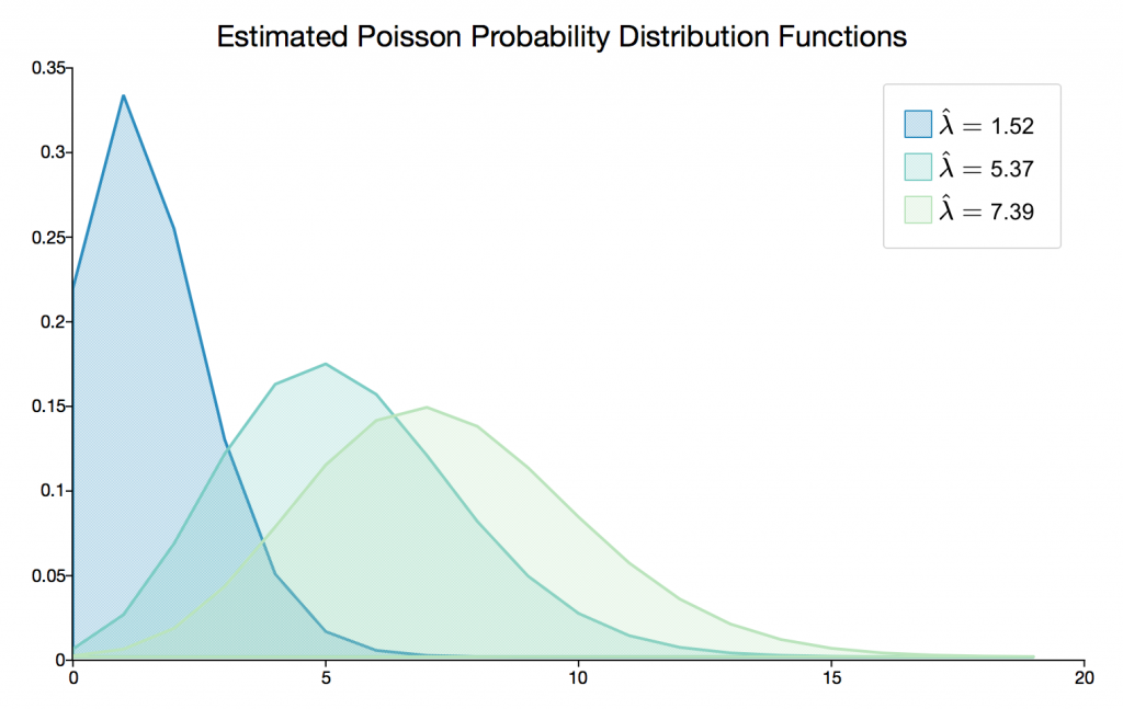
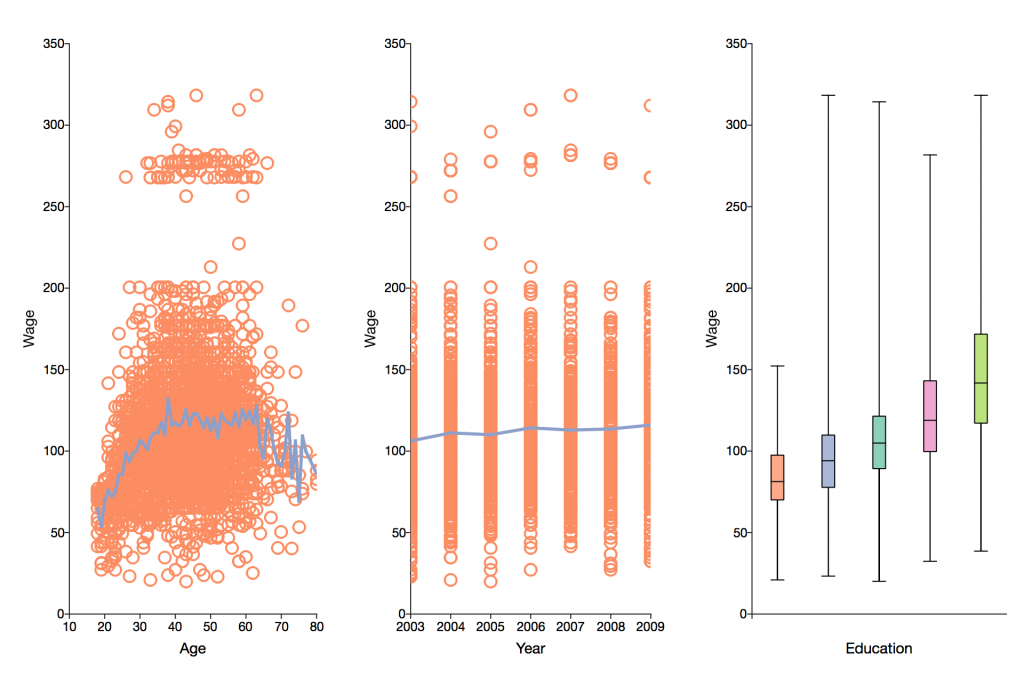
Convey insights from your data with modern, professional images.

New Color Palette Options and Defaults

GAUSS 18 color palette management tools allow you to apply professional color schemes to your graphics:

• Choose from over 30 built-in color palettes designed for optimal visual impacts.
  • Premade palettes available for sequential, quantitative and diverging data.
  • Colorblind friendly palettes available.

• Create your own palettes
  • Create sets of evenly spaced colors in HSL hue space.
  • Create sets of evenly spaced circular hues in the HSLuv system.
  • Blend colors to create custom color palettes.

Control graph canvas size programmatically

Easily produce and reproduce graphs that fit where you need them! The new GAUSS procedure `plotCanvasSize` adjusts plot canvas size programmatically based on specifications in centimeters, millimeters, inches or pixels.

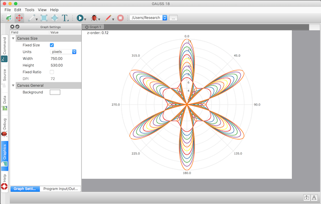
//Make this call before your plot to set the graph canvas
//to 750 px by 530 px as shown in the image above
plotCanvasSize("px", 750|530);

Other new features

string x_labels = { "Jan", "Feb", "Mar", "Apr", "May", "Jun" };
plotXY(x_labels, y);

• Easily pass in string arrays as 'X' labels to any 2-D graph such as scatter, XY, and others.
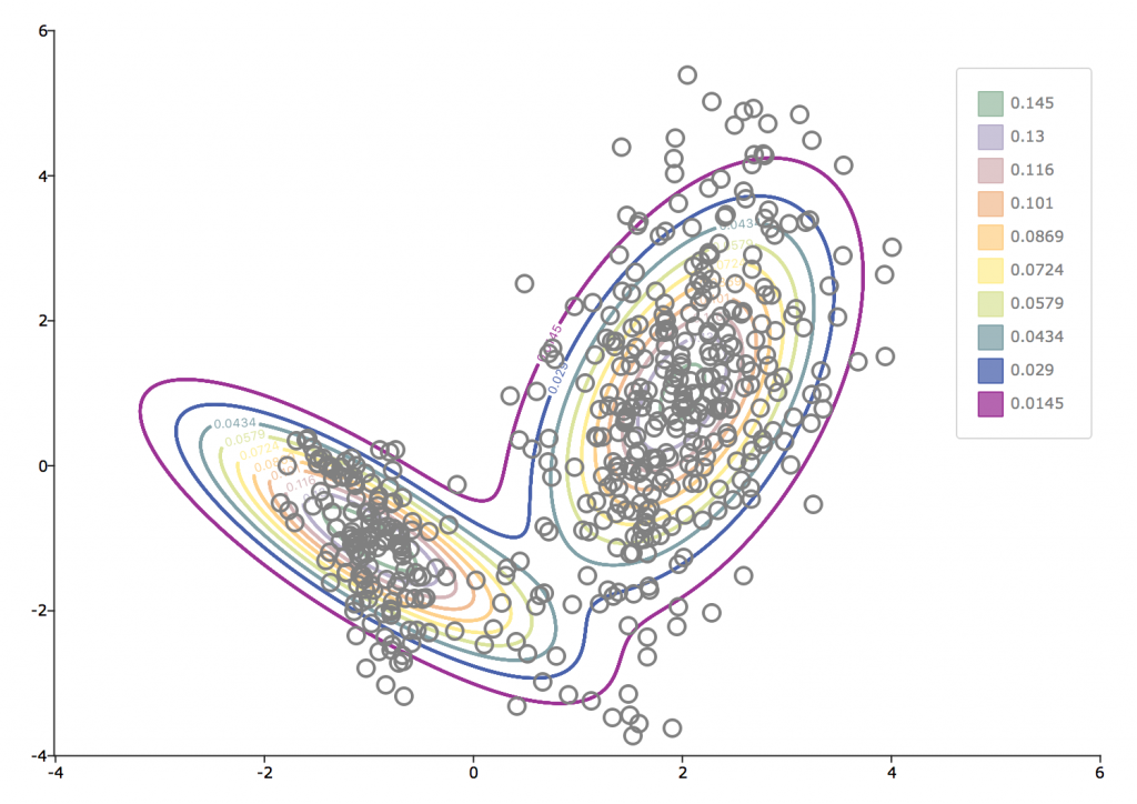
• Add any 2-D graph type, such as scatter plots, to contour plots.
• New function plotSetTicLabelFont to control the font, font-size and font-color of the X and Y tic labels.

New Functions to Increase Productivity

Increase your productivity with new GAUSS 18 features for efficient data navigation and organization. Uncover data insights quicker with new tools for searching, reorganizing, merging, and much more!

• New function innerJoin and outerJoin allow flexible matrix combining.

  ab = innerJoin(A, 1, B, 1);

  $$ A = \begin{bmatrix} 10001 & 21,021\\ 10029 & 32,183\\ 10012 & 17,151\\ \end{bmatrix} $$ $$ B = \begin{bmatrix} 10012 & 21\\ 10001 & 44\\ 10018 & 25\\ \end{bmatrix} $$ $$ {\xrightarrow[\text{columns }A_1\text{ and }B_1]{\text{innerJoin on}} \begin{bmatrix} 10001 & 21,021 & 44\\ 10012 & 17,151 & 21\\ \end{bmatrix}} $$
  

  ab = outerJoin(A, 1, B, 1);

  $$ A = \begin{bmatrix} 10001 & 21,021\\ 10029 & 32,183\\ 10012 & 17,151\\ \end{bmatrix} $$
  $$ B = \begin{bmatrix} 10012 & 21\\ 10001 & 44\\ 10018 & 25\\ \end{bmatrix} $$
  $$ \xrightarrow[\text{columns }A_1\text{ and }B_1]{\text{(left) outerJoin on}} \begin{bmatrix} 10001 & 21,021 & 44\\ 10029 & 32,183 & .\\ 10012 & 17,151 & 21\\ \end{bmatrix} $$
  
• Create block diagonal matrices using blockDiag.

  //'blockDiag' can create block matrices from 1, 2 or more input matrices
  d = blockDiag(A, B);

  $$ A = \begin{bmatrix} a_{11} & a_{12}\\ a_{21} & a_{22}\\ \end{bmatrix} \\ B = \begin{bmatrix} b_{11} & b_{12} & b_{13}\\ b_{21} & b_{22} & b_{23}\\ \end{bmatrix} $$
  $$ \xrightarrow[]{\text{blockDiag}} \begin{bmatrix} a_{11} & a_{12} & 0 & 0 & 0\\ a_{21} & a_{22} & 0 & 0 & 0\\ 0 & 0 & b_{11} & b_{12} & b_{13}\\ 0 & 0 & b_{21} & b_{22} & b_{23}\\ \end{bmatrix} $$
  
• Find whether a matrix, array or string array contains one or more elements from a list.

  //Find whether 'X' contains any elements in 'list'
  any = contains(X, list);

  $$ {X = \begin{bmatrix} M & married & NA\\ F & single & employed\\ F & married & employed\\ M & single & unemployed\\ \end{bmatrix}} $$
  $$ list = \begin{bmatrix} NA\\ ""\\ NaN \end{bmatrix} $$
  $$ \xrightarrow[]{\text{contains}} \begin{bmatrix}1\end{bmatrix} $$

   

• Find which observations (rows) match one or more elements with rowContains.

  //Find which rows in  'X' contain any elements from 'list'
  any = rowContains(X, list);

  $$ X = \begin{bmatrix} M & married & NA\\ F & single & employed\\ F & married & employed\\ M & single & unemployed\\ \end{bmatrix} $$
  $$ list = \begin{bmatrix} F\\ single \end{bmatrix} $$
  $$ \xrightarrow[]{\text{rowContains}} \begin{bmatrix} 0\\ 1\\ 1\\ 1 \end{bmatrix} $$

   

• Find which elements of matrix match one or more elements with ismember.

  //Find which elements in  'X' match any elements from 'list'
  match = ismember(X, list);

  $$ X = \begin{bmatrix} M & married & NA\\ F & single & employed\\ F & married & employed\\ M & single & unemployed\\ \end{bmatrix} $$
  $$ list = \begin{bmatrix} F\\ single \end{bmatrix} $$
  $$ \xrightarrow[]{\text{ismember}} \begin{bmatrix} 0 & 0 & 0\\ 1 & 1 & 0\\ 1 & 0 & 0\\ 1 & 1 & 0 \end{bmatrix} $$

   

• Easily collapse multidimensional arrays with the new squeeze function.

  //Remove any singleton dimensions from 'A'
  A = squeeze(A);

  $$ A \in \Re^{m,1,n} \xrightarrow[]{\text{squeeze}} A \in \Re^{m,n} $$
  
• Return the full path to the location of a program file regardless of location with __FILE_DIR

  //With your program and data in the same directory, __FILE_DIR
  //allows you to easily find your data regardless of your
  //working directory--greatly simplifies code sharing
  data_file = __FILE_DIR $+ "mydata.csv";
  
  //Prefer to keep your data in a different relative path?
  //No problem, __FILE_DIR works easily in this situation as well
  data_file = __FILE_DIR $+ "../data/mydata.csv";

• Delete specified columns from matrices with delcols.

  //Remove the 3rd and 5th columns from 'A'
  A = delcols(A, 3|5);

• Replace all matches of a substring within a larger string or string array with strreplace.

  //Regularize addresses: Avenue to Ave
  address = strreplace(address, "Avenue", "Ave");

  $$ address = \begin{bmatrix} \text{100 Main Ave}\\ \text{112 Charles Avenue}\\ \text{49 W State St}\\ \text{24 Third Avenue} \end{bmatrix} \xrightarrow[]{\text{strreplace}} \begin{bmatrix} \text{100 Main Ave}\\ \text{112 Charles Ave}\\ \text{49 W State St}\\ \text{24 Third Ave} \end{bmatrix} $$
  
• Array compatibility extended to erf, erfc, erfcinv, erfc, pdfn, and the power operator.

Speed Improvements

• Chained concatenation operations 2-4x faster
• X'Y for vector-vector case 15%-600% faster
• Inverse incomplete gamma function up to 10x faster

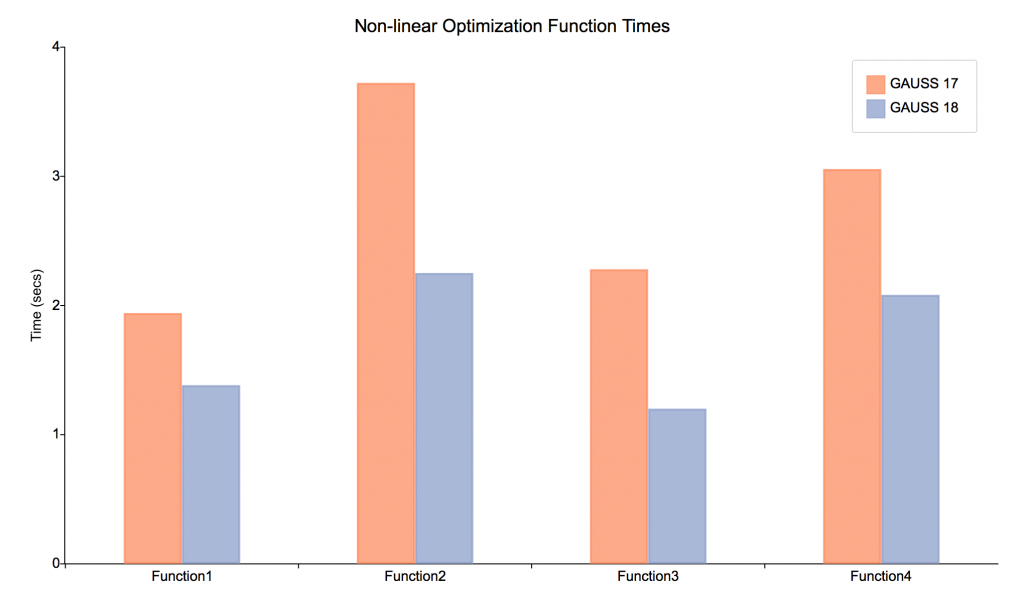
Experience improved speed for a number of fundamental computations in GAUSS 18 such as chained concatenation, vector-vector multiplication, and descriptive statistics.

Example nonlinear functions

In order to make the impact of the concatenation and indexing speed-ups more relevant, two of the nonlinear functions used to create the graph shown below the code.

	
proc fct_a(x);
    local f1,f2,f3;

    f1 = 3*x[1]^3 + 2*x[2]^2 + 5*x[3] - 10;
    f2 = -x[1]^3 - 3*x[2]^2 + x[3] + 5;
    f3 = 3*x[1]^3 + 2*x[2]^2 -4*x[3];
    retp(f1|f2|f3);
endp;

proc  fct_b(x);
    local ff1, ff2, ff3, ff4, ff5, ff6, ff7, P;
    P = 20;
    ff1 = 0.5*x[1] + x[2] + 0.5*x[3] - x[6]/x[7];
    ff2 = x[3] + x[4] + 2*x[5] - 2/x[7];
    ff3 = x[1] + x[2] + x[5] - 1/x[7];
    ff4 = -28837*x[1] - 139009*x[2] - 78213*x[3]
            + 18927*x[4] + 8427*x[5] + 13492/x[7]
            - 10690*x[6]/x[7];
    ff5 = x[1] + x[2] + x[3] + x[4] + x[5] - 1;
    ff6 = (P^2)*x[1]*x[4]^3 - 1.7837e5*x[3]*x[5];
    ff7 = x[1]*x[3] - 2.6058*x[2]*x[4];
    retp(ff1|ff2|ff3|ff4|ff5|ff6|ff7);
endp;

New mathematical functions

• besselk computes the modified Bessel function of the second kind; useful for the negative inverse gaussian distribution.
• rndRayleigh to compute Rayleigh distributed random numbers.
• gmmFit and gmmFitIV for estimation using the generalized method of moments.
• cdfTruncNorm, pdfTruncNorm, cdfLogNorm and pdfLogNorm.
• Optional mu, and sigma inputs for cdfn and pdfn
• Array support for erf, erfc, erfcinv, erfc, pdfn, power op.