Bayesian Estimation Tools
The GAUSS Bayesian Estimation Tools package provides a suite of tools for estimation and analysis of a number of pre-packaged models. The internal GAUSS Bayesian models provide quickly accessible, full-stage modeling including data generation, estimation, and post-estimation analysis. Modeling flexibility is provided through control structures for setting modeling parameters, such as burn-in periods, total iterations and others.
Features
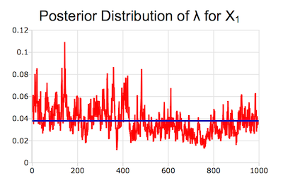
Posteriori Distribution of Lambda
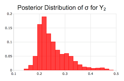
Posteriori Distribution of Sigma
GAUSS Bayesian internal models
- Univariate and multivariate linear models
- Linear models with auto-correlated error terms
- HB Interaction and HB mixture models
- Probit models
- Logit models
- Dynamic two-factor model
- SVAR models with sign restrictions
Individual modeling
Users can meet individual modelling needs by specifying key controls for the estimation algorithm including:
- Number of saved iterations
- Number of iterations to skip
- Number of burn-in iterations
- Total number of iterations
- Inclusion of an intercept
Data loading and data generation
Users may load data into GAUSS for estimation and analysis using standard intrinsic GAUSS procedures. However, in addition, the Bayesian Analysis Module includes a data generation feature that allows users to specify true data parameters to build hypothetical data sets for analysis.
Easy to interpret stored results
The Bayesian application module stores all results in a single output structure. In addition the Bayesian module graphs draws of all parameters and the posterior distributions for all parameters.
- Draws for all parameters at each iteration
- Posterior mean for all parameters
- Posterior standard deviation for all parameters
- Predicted values
- Residuals
- Correlation matrix between Y and Yhat
- PDF values and corresponding PDF grid for all posterior distributions
- Log-likelihood value (when applicable)
Example
Sample output report for probit model
Model Type: Probit regression model
*************************************************************
Possible underlying (unobserved) choice generation:
Agent selects one alternative:
Y[ij] = X[j]*beta_i + epsilon[ij]
epsilon[ij]~N(0,Sigma)
*************************************************************
Y[ij] is mvar vector
Y[ij] is utility from subject i, choice set j, alternative k
where	i = 1, ..., numSubjects
			j = 1, ..., numChoices
			k = 1, ..., numAlternatives - 1
*************************************************************
X[j] is numAlternative x rankX for choice j
*************************************************************
Pick alternative k if:
Y[ijk] > max( Y[ijl] )
for all k < mvar+1 and l not equal to k
Select base alternative if max(Y)<0
*************************************************************
Observed model:
*************************************************************
Choice vector C[ij] is a numAlternative vector of 0/1
beta_i = Theta'Z[i] + delta[i]
delta[i]~N(0,Lambda)
*************************************************************

Summary stats of independent data

*****************************************
Summary stats for X variables
*****************************************

        Variable             Mean              STD              MIN              MAX
              X1          0.33333          0.47538                0                1
              X2          0.33333          0.47538                0                1
              X3          0.33333          0.47538                0                1
              X4          0.28648          0.20641        -0.083584          0.71157
              X5         0.083333          0.59065               -1                1

*****************************************
Summary stats for Z variables
*****************************************

        Variable             Mean              STD              MIN              MAX
              Y1         -0.10328           1.1582          -6.1714           3.7266
              Y2         -0.23821           1.1428          -6.1295           3.2853
              Y3         -0.28473           1.2776          -5.4752             4.58

*****************************************
Summary stats for dependent variables
*****************************************

        Variable             Mean              STD              MIN              MAX
              Y1         -0.10328           1.1582          -6.1714           3.7266
              Y2         -0.23821           1.1428          -6.1295           3.2853
              Y3         -0.28473           1.2776          -5.4752             4.58

***********************************
MCMC Analysis Setup
***********************************
Total number of iterations:     1100.0
Total number of saved iterations:     1000.0
Number of iterations in transition period:     100.00
Number of iterations between saved iterations:     0.0000
Number of obs:    60.000
Number of independent variables:    5.0000
(excluding deterministic terms)
Number of dependent variables:    3.0000


********************************
MCMC Analysis Results
********************************

***********************************
Error Standard Deviation
***********************************
Variance-Covariance Means(Sigma)

        Equation               Y1               Y2               Y3
              Y1          0.20831         0.078641         -0.12772
              Y2         0.078641          0.26217        -0.078051
              Y3         -0.12772        -0.078051                1

***********************************
Error Standard Deviation
***********************************
Variance-Covariance Means (Lambda)

        Equation            Beta1            Beta2            Beta3            Beta4            Beta5
           Beta1         0.038024        0.0084823        0.0050414        -0.010463       -0.0044786
           Beta2        0.0084823         0.038058        0.0061952       -0.0098521        0.0017846
           Beta3        0.0050414        0.0061952         0.080755       -0.0086755         0.016158
           Beta4        -0.010463       -0.0098521       -0.0086755          0.10271        -0.010493
           Beta5       -0.0044786        0.0017846         0.016158        -0.010493         0.046216

***********************************
Theta for Z Equation     1.0000
***********************************

        Variable         PostMean          PostSTD
          Theta1          0.53176          0.43012
          Theta2          0.43195          0.35411
          Theta3        -0.011848       0.00015526
          Theta4          -2.0511          -1.9772
          Theta5           1.0605           1.1038

***********************************
Theta for Z Equation     2.0000
***********************************

        Variable         PostMean          PostSTD
          Theta1          0.90016          0.79037
          Theta2          0.37388          0.19278
          Theta3         -0.32424         -0.37066
          Theta4          0.69154          0.85307
          Theta5         -0.26623         -0.19126

***********************************
Theta for Z Equation     3.0000
***********************************

        Variable         PostMean          PostSTD
          Theta1         -0.24998          -0.2454
          Theta2         -0.22883         -0.19728
          Theta3        -0.043585         0.026509
          Theta4         -0.29718         -0.30046
          Theta5          0.52032          0.50741
System Requirements
System Requirements
Operating System
- Windows
- Mac
- Linux
Other Requirements
- GAUSS Version 13.1+
