GAUSSX Desktop Econometric Analysis for GAUSS
Funktionen
What is GAUSSX?

Gaussx incorporates a full-featured set of professional state-of-the-art econometric routines that run under GAUSS. These tools can be used within Gaussx, both in research and in teaching. Alternatively, since the GAUSS source is included, individual econometric routines can be extracted and integrated in stand-alone GAUSS programs.
Gaussx provides an environment that makes econometric programming a joy. For example,
ols y c x1 x2;
does ordinary least squares, while
mcmc z1 c z3 z4;
userproc = &g_tobit;
does a Bayesian estimation of a Tobit model using Markov Chain Monte Carlo.
Gaussx provides for linear and non-linear optimization with and without parameter constraints. A full set of econometric models, estimation routines and tests are supported, including: automatic differentiation, multivariate binomial probit, VARMA process, time series analysis, LDV models, GARCH models, exponential smoothing, X12 seasonal adjustment, non-parametric analysis, neural networks, wavelets, forecasting, Kalman filter, stochastic volatility, robust estimation, Bayesian estimation, cluster analysis, financial tools, econometric tests, Monte Carlo simulation and statistical distributions.
Gaussx is designed for econometricians and financial analysts and has been continuously upgraded over 15 years. The open source paradigm allows econometricians to use GaussX routines as templates for their own code.
Linear Estimation Methods
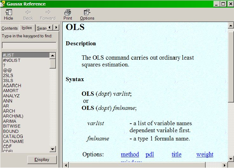
Linear models include AR, ARCH, OLS, POISSON, QR, SURE, VAR, 2SLS, and 3SLS. Descriptive statistics, elasticities, automatic treatment of missing values, weighted analysis and White or Newey-West robust standard errors are standard. Lag specification such as y(-1) is supported, as are PDL structures. Diagnostics for single equations include Godfrey's test for residual serial correlation, Ramsey's RESET test for functional form, Jarque-Bera's test for normality of residuals, Breusch-Pagan test for heteroscedasticity, and Chow's test for stability.
Non-linear Estimation Methods
Non-linear models include FIML, GMM, NLS, and ML. Step-algorithms include BFGS, BHHH, DFP, GA (Genetic Algorithm), GAUSS, NR, and SA (Simulated Annealing). Step size methods include line search and trust region. Both the White and Newey-West robust estimators are supported. The defaults used during non-linear estimation can be altered heuristically during execution, or through a script file. Gradients, Hessian, and Jacobian are estimated numerically as the default; however they can be written as a procedure by the user. The maximum likelihood (ML) procedure permits the estimation of any specified likelihood - Gaussx includes examples for non-linear ARCH, FRONTIER, E_GARCH, FMNP, GARCH, GARCH-M, MGARCH, LOGIT, MNL, MNP, MSM, NPE, POISSON, PROBIT, SUR, SV , TOBIT, 2SLS and 3SLS. Coefficient restrictions can be imposed with PARAM, and investigated using ANALYZ, which can be used following either linear or non-linear estimation. Descriptive statistics, automatic treatment of missing values, and weighted analysis are standard.
Constrained Optimization
Constrained optimization is supported under FIML, GMM, ML and NLS. The parameter constraints can be linear or non-linear. The estimation is undertaken using sequential quadratic programming. The constrained confidence region for any specified confidence level for each parameter is calculated.
Automatic Differentiation
A choice of numeric, analytic, or symbolic derivatives is available for FIML, ML and NLS. The default method of deriving gradients and Hessians is numeric, using finite differencing. Analytic derivatives are specified by the user, while symbolic derivatives are calculated using the automatic differentiation capability of Maple 9. Symbolic gradients and Hessians can be saved as procedures and reused. Symbolic gradients work only for Gaussx for Windows, and requires Maple 9.
Time Series Analysis
A complete range of time series analysis is available under Gaussx, including ARMA, ARIMA and ARFIMA for single equations, and VAR and VARMA for multiple equations. ARIMA includes full identification, estimation and forecasting with graphical presentation. Systems of transfer functions can be specified, with a separate moving average structure for each equation. Markov switching models (MSM) include AR components and non-linear state equations. Spectral analysis is also supported
LDV Models
Linear LDV models include binomial probit, multinomial logit, and ordered logit and probit; in each case the marginal effects and elasticities, and their variances, evaluated at the mean, are available. For both probit and logit, Mills ratio is available allowing correction for selection bias. Heckman's two step procedure (HECKIT) incorporates Greene's covariance correction. Non linear multinomial logit and probit (MNL and MNP) are available using ML; for the latter, high dimensional integration is carried out either exactly using the Gauss CDFMVN function, or through simulation using the smooth recursive simulator. Double-bounded (DBDC) models are also supported. For models with large number of alternatives, feasible multinomial probit (FMNP), which does not require parameterization of the covariance matrix, is available for both ranked and non-ranked data.
GARCH Models
A variety of Arch and Garch models are supported; these include linear ARCH, single equation non-linear ARCH, AGARCH, EGARCH, FIGARCH, GARCH, IGARCH, PGARCH and TGARCH. Residuals can be distributed normal, Student-t, or GED. Garch in the mean, leverage options, and MA residuals are all supported. Stability and positive variance is secured using the constrained optimization facilities.
Multivariate GARCH (MGARCH) estimated over a system of equations, with the option of weakly exogenous variables, is also supported, under both the VEC and BEKK formulation. MGARCH-M is also available.
Exponential Smoothing
Methods include single, double, Holt-Winters, and seasonally additive or multiplicative Holt-Winters. Smoothing parameters can be user specified or optimally estimated by Gaussx.
Denoising
Denosing of signals and time series is accomplished using wavelet shrinkage methods. Thresholds include universal, minimax and SURE.
Non-parametric Analysis
Non-parametric and semiparametric analysis under Gaussx permits the estimation of the window width and the weights in the semiparametric index using cross validation under maximum likelihood. For the single index case, the FFT is used to speed calculation. Conditional response coefficients are determined for the density, conditional mean, discrete and smeared case.
Neural Networks
The hidden and output weights in a feed forward network with a single hidden layer are estimated using non-linear optimization, rather than back propagation. Transfer functions include Arctan, Gaussian, Halfsine, Linear, Sigmoid, Step, and Tanh. Output processing includes levels, density, and maximum.
Forecasting
Static and dynamic forecast values and residuals are available for all estimations. Systems of non-linear equations can be solved statically or dynamically. An impulse response function is available for VAR models. OLS forecasts also include prediction error, studentized residuals, DFFITS and DFBETAS. GARCH forecasts include conditional variance, QR forecasts include probabilities and category, and ARFIMA forecasts include both naive and best linear predictor.
Kalman Filter
Analysis with the Kalman Filter allows for the estimation of state vectors, with smoothing, time varying transition matrices (ie. each element is a function), and the estimation of the elements of the Kalman matrices using ML. Stochastic Volatility models (SV) are estimated using quasi ML based on a Kalman Filter model.
Robust Estimation
Robust estimation of linear models when the distribution of the residual is unknown is undertaken using Quantile Regression (interior point algorithm), as well as using reiterated weighted least squares for Least Absolute Deviation, Huber's t Function, Ramsay's E Function, Andrew's Wave Function, and Tukey's Biweight. The parameter covariance matrix is estimated using bootstrapping.
Data Handling and Conversion
Memory allocation and all file control is handled automatically. Data size for non-AR estimation is limited by disk capacity only. External data can be imported as delineated ASCII, packed ASCII, binary, Lotus, Excel, Gauss data files, Gauss format files, and Gaussx save files. Data can be exported as ASCII, binary, Gaussx or Gauss data files. Under Windows, import/export is available for Lotus, Excel, Quattro, Dbase, Symphony, Paradox, Foxpro, Clipper and both delineated and packed ASCII. Variables in a Gaussx dataset can be user selected with the KEEP or DROP commands.
Data Creation and Transformation
Data transformation (GENR, FEVAL) permits the use of all Gauss operations and all the Gauss functions, such as FFT, all Gauss distributions, random number generators, etc. Thus all the power of Gauss is available in Gaussx. However sample selection (SMPL) makes coding far simpler, and data input/output is transparent. Stochastic data can be created using 13 distributions with DGP, and data can be filtered with FILTER.
Descriptive Statistics
Each Gaussx variable can have a descriptor (comment) associated with it. Data description includes means, standard deviations, minimum and maximum, sum, covariance and correlation matrices, autocorrelogram, partial autocorrelogram, and singular value decomposition (including variance decomposition). Divisia indices, seasonal adjustment (including Census X12), and principal components are supported. TABULATE (which replicates PROC TABULATE in SAS) tabulates data across two class variables by count, mean, SD, variance, minimum, maximum, sum and percent (row, column and total). This also permits standard frequency and crosstab.
Cluster Analysis
Cluster analysis creates an hierarchical cluster tree of the data, and optionally graphs the tree - a dendrogram. Five distance metrics and four linkage methods are available.
Financial Tools
Financial tools include PV, FV,AMORT and MCALC for amortization and loan caluclations, FRONTIER (Markowitz efficient frontier), and a full range of single and multi equation GARCH estimation tools.
Econometric Tests
The TEST command includes the likelihood ratio test, the Chow test for stability, Ljung-Box Q test for AR, Engle's LM test for Arch, Breusch-Pagan amd Goldfeld-Quandt tests for homoscedasticity, F-test for linear restrictions, CUSUM and CUSUM-squared tests for stability, Granger's causality test, Dickey-Fuller test for unit roots, Engle-Granger and Johansen tests for cointegration, Belsley, Kuh and Walsh test for collinearity, Thiel's decomposition of two vectors, Hausman's specification test, Lagrange Multiplier test, and Davidson and MacKinnon's J-Test for non-nested estimations.
Simulation
Monte-Carlo simulation can be carried out over a block of code, using both bootstrap and jackknife methods. For Bayesian analysis, Markev Chain Monte Carlo is carried out over user supplied distributions and priors - examples include continuous, LDV and censured models. Output for the selected variables is shown dynamically on the screen, and final output includes cumulants and quantiles.
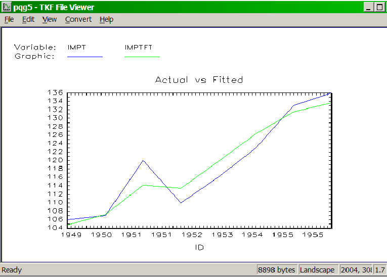
Graphics
Graphical output (PLOT, GRAPH, COVA) is available either in text mode or in graphic mode, in mono or color. Gaussx has full support for all Gauss PQG routines. Line and scatter graphs/plots are supported. Printed output is available in both text and graphic mode. Interative GraphiX (IGX) is supported directly from the Gauss tools menu.
Distributions
A set of procs for evaluating density functions is included, which can be used from Gauss or Gaussx; these provide the PDF, the CDF, the inverse CDF and random sampling from the beta, binomial, Cauchy, central and non central chi-squared, exponential, central and non-central F, gamma, geometric, Gumbel, hypergeometric, logistic, log normal, negative binomial, Laplace, normal, truncated normal, Pareto, Pearson, poisson, central and non-central t, uniform, and weibull distributions. Sampling from a truncated multivariate normal, multivariate t, and Wishart distribution, as well as sampling with and without replacement are also available.
Programming Features
All Gauss commands, logical goto, DO loops, and Gauss procs can be used within a Gaussx file. In addition, Gaussx provides a number of programming commands; these include macro definitions for formulae, LOOP control for multisectored data, GROUP control (like BY in SAS) and recursive LIST names. A timer control is available to simulate realtime analysis.
Symbolic Algebra
Symbolic algebra can be used for symbolic differentiation and integration, exact linear algebra, and equation solving. Gaussx uses Maple and/or Mathematica to permit Gauss to undertake symbolic manipulation. Simply include the Maple/Mathematica statements within the command file, select the statements, and click the Maple or Mathematica button. This works only for Gaussx for Windows, and requires MapleV, rev 4 or higher or Mathematica, rev 3 or higher.
Mixing GAUSS and GAUSSX
Gauss statements can be included within the command file. Gaussx variables can be made global (FETCH), and global variables can be stored in the Gaussx workspace (STORE). Thus maximum flexibility is achieved by being able to mix Gauss and Gaussx commands. User written procs can be included within Gaussx formula definitions. In addition, most Gauss application modules can be run directly from a Gaussx file.
Extending GAUSSX
The complete source code, written in Gauss, is included. Thus even if you don't want all the features of Gaussx, you can extract a particular procedure and use it in your own Gauss programs -- procedures such as inverse cumulative normal density function, Gibbs sampling, smooth recursive simulator (GHK), multivariate normal rectangle probabilities for any dimension, random sampling from a multivariate truncated distribution, maximum entropy estimation, quasi random sequences, bitwise arithmetic and more. And because of its modular design, you can also add your own procedures to Gaussx, or modify any Gaussx procedure to fit your requirements.
Project Management
Windows Project Control Screen
Project management is provided for Gaussx for Windows, with up to 100 separate applications, each associated with different file names and paths. Gaussx is network compatible - thus on a network, each client has its own project and configuration file. Project management can also be used to manage pure Gauss applications.
Help Facilities
During execution of a command file, pop-up help is available to explain the current screen, using Alt-H. Under Windows, context sensitive help (F1) is available to provide the complete syntax of each Gaussx command.
Neu in Gaussx 10
GAUSS 11 Support
Gaussx has been updated to support the new GAUSS 11 interface, and incorporate the new functionality of GAUSS 11.
Copulas
A copula is used in statistics as a general way of formulating a multivariate distribution with a specified correlation structure.
Example:
let rmat[3,3] = 1 .5 .2 .5 1 .6 .2 .2 .6 1;
q = copula(1000,rmat,1);
v1 = normal_cdfi(q[.,1], 0, 1);
v2 = expon_cdfi(q[.,2], 2);
v3 = gamma_cdfi(q[.,3], 1.5, 2.5);
q is a 1000x3 copula matrix with a Kendal Tau correlation structure given by rmat. This copula is then used to create three correlated random deviates drawn from the normal, exponential and gamma distributions.
CORR
Computes a correlation matrix for different correlation types - Pearson, Kendall Tau b and Spearman Rank.
MVRND
Creates a matrix of (pseudo) correlated random variables using specified distributions.
Example:
dist = "normal" $| "expon" $| "gamma";
let p[3,3] = 0 1 0 0 1 0 0 0 1.5 2.5 0 0;
let rmat[3,4] = 1 .5 .2 .5 1 .6 .2 .6 1;
s = mvrnd(1000, 3, dist, p, rmat, 2);
This example creates s, which is a 1000x3 matrix of correlated random variates consisting of the three distributions shown in dist, with the correlation structure specified by the Spearman rank matrix rmat.
STEPWISE
In a situation where there are a large number of potential explanatory variables, STEPWISE can be useful in ascertaining which combination of variables are significant, based on the F statistic. It includes the capability of scaling data, and expanding a given data set to include cross and/or quad terms. This is an exploratory, rather than a rigorous tool.
Example:
oplist = { .4 .25 };
indx = stepwise(y~xmat, 0, oplist);
{xnew, xname} = xmat[.,indx];
This example shows how a stepwise regression is applied to a matrix of potential explanatory variables xmat, using .4 and .25 for the F statistic probability of entry and exit.
Latin Hypercube Sample - LHS
LHS has the advantage of generating a set of samples that more precisely reflect the shape of a sampled distribution than pure random (Monte Carlo) samples. The Gaussx implementation provides standard LHS, nearly orthogonal LHS, and correlation LHS.
Example:
n = 30; k = 6;
fill = 0; ntry = 1000; crit = 2;
dsgn = fill | ntry | crit;
p = lhs(n,k,dsgn);
x = weibull_cdfi(p,1,1.5);
In this example, a 30x6 nearly orthogonal Latin Hypercube Sample is derived using the best condition number as the criteria. This creates a 30x6 matrix of probabilities, which are then used to create a set of Weibull distributed variates, each column being orthogonal to every other column.
STATLIB - Statistical Distribution Library
The STATLIB library has been updated; it now includes 51 continuous distributions, and 9 discrete distributions. This library can be used independently of Gaussx, or as part of Gaussx - for example in an ML context.
In the context of ML estimation, the parameters of a particular distribution can be estimated from a set of data, or a parameter can be replaced by a linear or non-linear function, whose parameter can also be estimated. Threshold estimates for distributions where the data is non-negative is also supported.
Example:
x = seqa(0,.2,6);
a = 2; b = 4;
p = beta_pdf(x,a,b);
param b0 b1;
value = .1 1 ;
FRML eq1 v = b0 + b1*x;
FRML eq2 llfn = chisq_llf(y,v);
ML (d,p,i) eq1 eq2
method = nr nr nr;
The first example shows pure GAUSS code for estimating the pdf for a beta distribution. The second shows how the parameters of a function which is used to replace a parameter in a distribution can be evaluated.
Systemvoraussetzungen
System Requirements
Gaussx for Windows runs as a 32-bit Windows application when it runs under a 32-bit version of GAUSS, and as a 64-bit application when run under a 64-bit version of GAUSS.
Gaussx can be run on a single machine or on a network, under either Windows, Mac OSX, Linux or Unix. Gaussx supports GAUSS 6 through 11.
GAUSSX for UNIX, Linux and MAC runs in Terminal mode. Networking is built in, so that individuals will each have their own configuration file. The econometric specifications for the Unix version is identical to the Windows version. Gaussx for Unix has been designed to be machine independent by writing the entire package in Gauss. Thus, if your Unix machine runs Gauss, it will run Gaussx.