Visualizations of Gaussian Results
The following examples illustrate how to visualize the results obtained by Gaussian. For the visualization either GaussView or Chem3D is used.
GaussView
Manipulating and Modeling Large Molecules
GaussView 5 provides features for every phase of studying large molecular systems, from importing molecules from PDB files, through modifying structural features and setting up ONIOM calculations in Gaussian, to viewing and plotting the final results. GaussView can also import many other popular structure exchange formats.
GaussView 5 provides comprehensive support for importing and working with structures from PDB files:
- Select the desired structure(s) from multi-structure files.
- Add hydrogen atoms to all atoms automatically or manually according to user preference.
- Selectively add hydrogen atoms to one or more residues, chains, helices or other defined structural entities.
- Highlight/select atoms in individual residues or secondary structures.
- Quickly determine residue membership for any atom selected with the mouse.
- Easily assign atoms to ONIOM layers based on a variety of flexible criteria.
- Retain residue information within Gaussian 09 calculations and retrieved Gaussian 09 results.
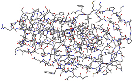
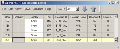
The molecule above is HIV protease (Type 1) complexed with an inhibitor, with the latter displayed in ball-and-stick format. The dialog below is the PDB Residue Editor which provides a convenient way to interact with large molecules on a per-residue basis. Here we have sorted the residues by name and are now working with the atoms in the inhibitor. We will go on to use other tools to assign atoms to ONIOM layers.
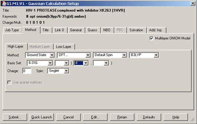
We set up and run a Gaussian 09 calculation using the dialog below. We check the box selecting an ONIOM calculation and use the per-layer components of the Method panel to select the desired model chemistries. When we are ready, clicking the Submitbutton will initiate the Gaussian 09 calculation.
The Gaussian 09 ONIOM method is typically used to study large molecules of biological interest. GaussView 5 contains several methods for assigning atoms to the distinct layers used by ONIOM to divide the problem into regions of differing modeling accuracy/computational cost. The illustration below depicts the familiar Layer Selection Tool. We are using it to select specific residues within the complex.
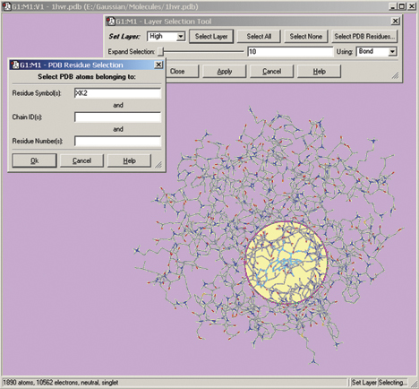
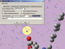
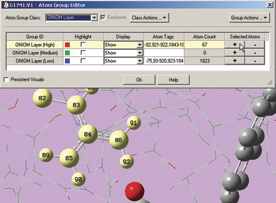
The next two illustrations depict features introduced in GaussView 5 which we use to add residues in close proximity to the inhibitor to the High layer. First, we zoom in on the relevant part of the complex, and select a nearby atom with the mouse (middle illustration). Using the Atom Selection Editor’s Expand Selection slider, we expand the selection to include the entire residue containing that atom. Once the desired atoms are selected, we use the Atom Group Editor to quickly add them to the desired ONIOM layer by clicking on the plus sign button in the corresponding Selected atoms column. We can continue to select and add nearby residues in this way until the High layer is complete.
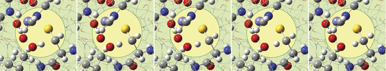
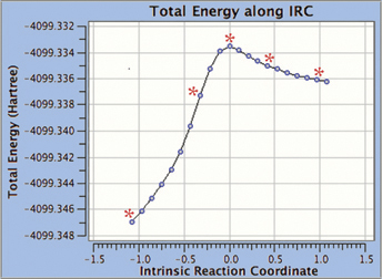
GaussView 5 can display plots and animations from Gaussian 09 studies of such systems. The 5 frames below depict structures from the reaction path for a proton transfer within nonheme iron enzyme isopenicillin N synthase (5368 atoms). We located the transition structure and then ran an IRC calculation. The corresponding points on the energy plot have been marked with asterisks. We suppressed the display of Low layer atoms in the highlighted region for clarity using GaussView’s Atom List Editor.
Building Molecules: Easier Than Ever
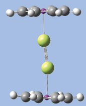
GaussView has provided powerful molecule building features for some time, and GaussView 5 significantly expands that repertoire. We will introduce several of them by demonstration as we build the diuranium metallocene system featured in the lower left of this booklet’s cover: U(II)2(?8-COT)2 [bis(?8-cyclooctatetraene) diuranium]. This molecule has D8h symmetry. The molecular orbitals predicted by the Gaussian calculation are also displayed in the cover illustration.
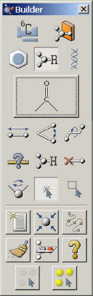
Here is the procedure:
- GaussView 5 provides a palette of the most commonly-used ring fragments. However,
the eight-membered ring included there is cyclooctane (chair configuration).
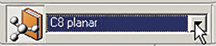
We need a planar 8-carbon ring. We’ve needed this before, and we saved the structure
in our custom fragment library. We select it from the building toolbar and click
in the view window to add it.
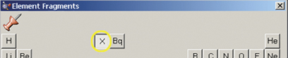
- Choose the dummy atom from the Element Fragments palette (atomic symbol X):
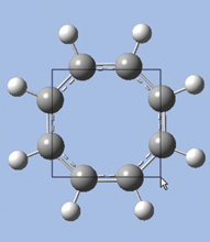
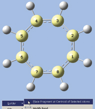
- We now want to select all of the carbon atoms. One quick way is to use GaussView
5’s new rubberband selection mode. In the view window, hold down the R key and
drag the mouse, creating a box that touches all carbon atoms (see the first illustration
at the right). When you release the mouse button, the selected atoms turn yellow
(as in the second illustration at the right).
- Right click in the view window, and then select Builder? Place Fragment at Centroid of Selected Atoms from the context menu. A magenta-colored dummy atom will appear in the center of the ring.
-
Click on the Rebond icon; this adds bonds from the dummy atom to all 8 carbons.

-
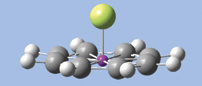
Click on the Add Valence button and then on the dummy atom. A hydrogen atom will appear bonded to the dummy atom perpendicular to the plane of the ring. Change the hydrogen atom to a uranium atom. The molecule will now appear as in the illustration below.

-
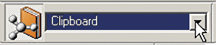
Select the entire molecule. A quick way to do so in GaussView 5 is to press the A key when the view window is active. Then, type Ctrl-C or Command-C, copying it to the clipboard. Any structure on the clipboard is always available in the custom fragment menu. Select the Clipboard item, and then click in a convenient location to add another monomer to the view.
- Holding down the Alt key to limit mouse actions to the new fragment, move it into the approximate desired position. Hint: placing the second U atom inside the first one makes it easier to position the two rings parallel to one another. Afterwards, draw the second fragment away from the first.
-
Add a triple bond of length 2.24 Å. Then adjust the X-U-U-X dihedral angle to 180°.
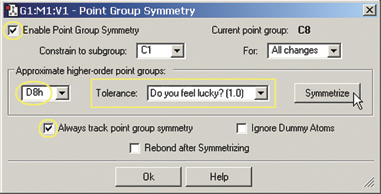
- The final step is to impose the proper symmetry on the molecule via the Point
Group Symmetry dialog (on the Edit menu). When we enable point group symmetry,
the molecule has C1 symmetry. We set the Tolerance to its loosest level, chooseD8h from
the popup and then click the Symmetrize button to impose this symmetry on the
molecule (see the dialog at the right). The structure is now complete.
The following illustrations depict other advanced building features offered by GaussView 5.
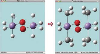
In the illustration below, we see another aspect of GaussView 5’s point group symmetry feature. Here we have enabled continual tracking of point group symmetry for this bridged iron complex (D2h). When we click on the hydrogen atom above the left iron atom with the tetrahedral carbon atom selected, a methyl group is automatically added to all four symmetry-equivalent hydrogen atoms.
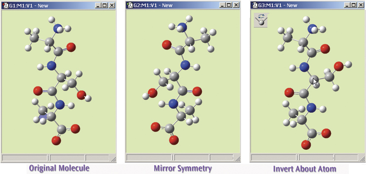
The final illustration shows the operation of the Mirror Symmetry and Invert About Atom features, which flips the symmetry of the entire molecule or inverts it about a selected atom (respectively). The original molecule is on the left. The middle view shows this tripeptide species after using Mirror Symmetry. The view on the right shows the result of using Invert About Atom by clicking on the central carbon atom (indicated with the cursor).
Examining Molecular Orbitals and Other Surfaces

Examining molecular orbitals and the spatial distribution of other molecular properties is useful for many purposes. MOs can provide important insight into bonding and other chemical properties. Visualizing them can also be useful for modifying the initial guess for a subsequent Gaussian 09 calculation and for selecting the active space for the CASSCF method.
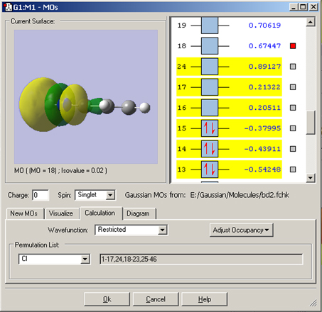
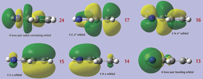
In this example, we consider the orbitals for C3H4NH. We plan to run a CASSCF calculation on this molecule using an active space of 6 orbitals and 6 electrons. Since we are interested in the n–p* transition, we need to select the p and p* orbitals corresponding to the C=C and C=N bonds, the bonding orbital corresponding to the nitrogen lone pair, and another orbital which correlates with it (labeled the “radial correlating” orbital at the top right).
We use the GaussView 5 MOs dialog’s ability to examine multiple MOs: the LUMO (16), HOMO (15) and nearby orbitals. We locate the p, p* and N lone pair bonding orbitals in 5 adjacent orbitals about the HOMO and LUMO: orbitals 13-17. However, neither orbital 12 nor orbital 18 exhibit the node located within the plane of the molecule which will characterize the correlating orbital (orbital 18 is visible in the illustration below). We continue examining higher orbitals, and locate the one we want at orbital 24. We then reorder the orbitals. Since this system is closed shell, we do not need to move any electrons between orbitals, but the dialog allows you to do so if appropriate.
The final set of orbitals chosen for the active space appear below:
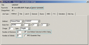
This orbital reordering is carried over to the Gaussian job when we check the Use Orbitals Selected in MOs Dialog box on the Method panel, and the relevant keyword and additional input section are added automatically. We also set the characteristics of the active space for the job using the fields provided:
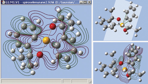
The orbitals we just examined were visualized as transparent surfaces, allowing us to see the atoms in the molecule at the same time. There are several other modes for displaying such volumetric results. For example, the figure at the top left displays contours on the plane through an MO of spiroselenurane. This feature is highly customizable; the two smaller images illustrate selecting a different projection plane—defined by the three central atoms and the included ring—and the resulting contour display:
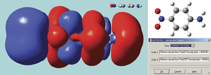
The surface below in solid mode. It is a difference density between the excited state and ground state total electron densities for para-nitroaniline, computed by GaussView 5 using its internal cube operations facility (see the dialog). This molecule has a planar geometry; we optimized the structure using the B3LYP/6-31G(d) model chemistry. The excitation calculation was performed in Gaussian 09 using the LC-BLYP functional of Hirao, a long-range corrected functional which correctly treats charge-transfer states, a problem with which traditional functionals often have trouble. The resulting surface shows the charge transfer in this excitation, with electrons moving toward the NO2 group (left side of the molecule).
Finally, the illustration below uses the mapped surface feature. In this case, the electron density surface is painted with the electrostatic potential for 21-thiaporphyrin.
![]()
Reference: E. P. Zovinka and D. R. Sunseri, J. Chem. Ed. 79 (2002) 1331.
Preparing Gaussian 09 Calculations
GaussView 5 provides comprehensive support for all Gaussian 09 features via a wide variety of facilities for setting up specific calculation types graphically. It gives you the ability to:
- Assign atoms to ONIOM layers in several ways (as we saw). GaussView 5 also makes it easy to specify molecular mechanics atom types and charges.
- Reorder and repopulate MOs for CASSCF and other jobs.
- Add and redefine redundant internal coordinates.
- Specify frozen atoms/coordinates during geometry optimizations.
- Set atom equivalences for STQN transition state optimizations (see below).
- Define fragments for fragment guess/counterpoise calculations, including assigning fragment-specific charges and spin multiplicities.
- Select atoms for normal mode analysis (frequency calculations).
- Specify atoms for NMR spin-spin coupling.
- Build unit cells for polymers, 2D surfaces and crystals for use in periodic boundary conditions (PBC) calculations.
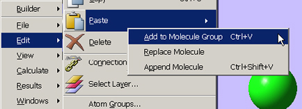
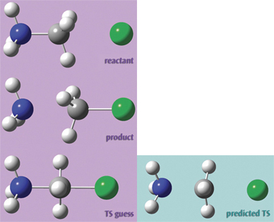
We used the molecules at the right in a transition structure optimization for this SN2 reaction. Setting it up in GaussView 5 was very easy. First, we built the reactant. We then copied the structure into a second frame within the same molecule group using Edit? Copy? Add to Molecule Group. This results in a second molecule with identical atom ordering, as required by Opt = QST3:
We go on to transform that structure into the product. Hint: Rotating to an end-on view is an easy way to ensure proper fragment alignment and hydrogen atom positioning:
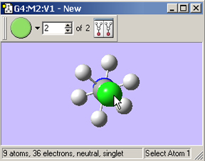
Finally, we set up the transition state guess structure in the same way.
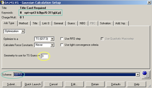
The Gaussian Calculation Setup dialog provides a menu-based interface to Gaussian 09 keywords and options. The dialog below shows the settings used for the TS optimization:
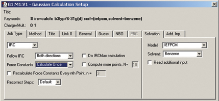
The Gaussian Calculation Setup dialog automatically displays related settings for whatever selections you make, and the various tabs provide access to all major G09 features (cf. the example below for an IRC calculation in solution):
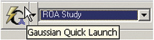
The setup dialog for the QST3 job also illustrates another Gaussian 09 convenience feature of GaussView 5: calculation schemes. Selecting an item from the Scheme menu causes a set of saved keywords and options to be applied to the current job in a single step. Using schemes in conjunction with the Gaussian Quick Launch feature allows you to initiate a calculation on the current molecule with a single click:
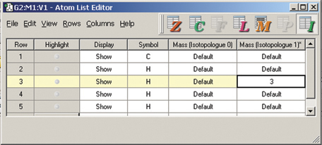
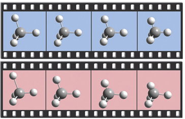
The dialog below shows GaussView 5’s facility for defining isotopes for the various atoms in the molecule, including multiple isotopologues. They can be used within subsequent frequency analyses. In this example, two isotopologues are defined: one with the standard (most abundant) isotopes, and a second with tritium substituted for one of the hydrogen atoms. The animations at the right illustrate the resulting change in the symmetric H stretch normal mode; the tritium-substituted atom is the one with the elongated motion in the frames with the rose background.
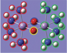
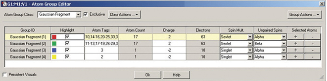
The illustrations below depict GaussView 5’s support for defining fragments for use in Gaussian 09 counterpoise, fragment guess and related calculations. We are using the Atom Group Editor to define fragments and set fragment-specific charges and spin multiplicities in order to model antiferromagnetic coupling with Gaussian 09. See this web page for a detailed discussion of this calculation: www.gaussian.com/g_tech/afc.htm.
Chem3D
Chem3D
Neben dem Standardprodukt GaussView, ist es auch möglich, die Ergebnisse von Gaussian-Modellierungen mit der Software Chem3D zu visualisieren. Die Vorgehensweise beschreibt der Artikel "Visualizing Gaussian's Results with Chem3D".
Ausführliche Informationen zu Signals ChemDRaw und Chem3D erhalten Sie auf unseren Signals ChemDraw-Produktseiten.